\( \def\AA{{\bf Å}} \def\ii{{ 𝟙}} \def\bold#1{{\bf #1}} \)

Roehr-Lab

We develop and apply theoretical methodologies suitable for investigating aggregation-induced functions in supramolecular structures in both the ground and excited states. In particular, we study how supramolecular systems can facilitate (photo-)catalytic reactions and how structural motifs affect charge and exciton transport. We employ new atomistic dynamics simulation techniques, allowing us to gain insight into the mechanistic details of these processes. Furthermore, we aim to understand how molecular aggregates are formed and, consequently, how the formation of desired structural motifs can be controlled.

Dr. Merle I. S. Röhr

Google Scholar

Telephone: +49 931 31 88832

E-Mail: merle.roehr@uni-wuerzburg.de

Fragment Molecular Orbital Configuration Interaction Methodology for the Description of Correlated States in Extended Molecular Aggregates

Project of

Anurag Singh

Project

Symbolic-CI Software Development

WebSlides Files

Singlet Fission model for Trimer

WebSlides Files

SFast Software Development for Dimer

WebSlides Files

SFast , B-N doping and optimisation

WebSlides Files

Software Development for Fragment Molecular Orbital base Configuration Interaction

Branching Diagram approach to make configuration state function

Number of electrons 6
Select the final \(S\) (Spin) 0
Select the pathway of \(S\) for combination of electrons 0
Select the pathway of \(M\) (High Spin State) 0
Select final \(M\) 0


WaveFunction Construction

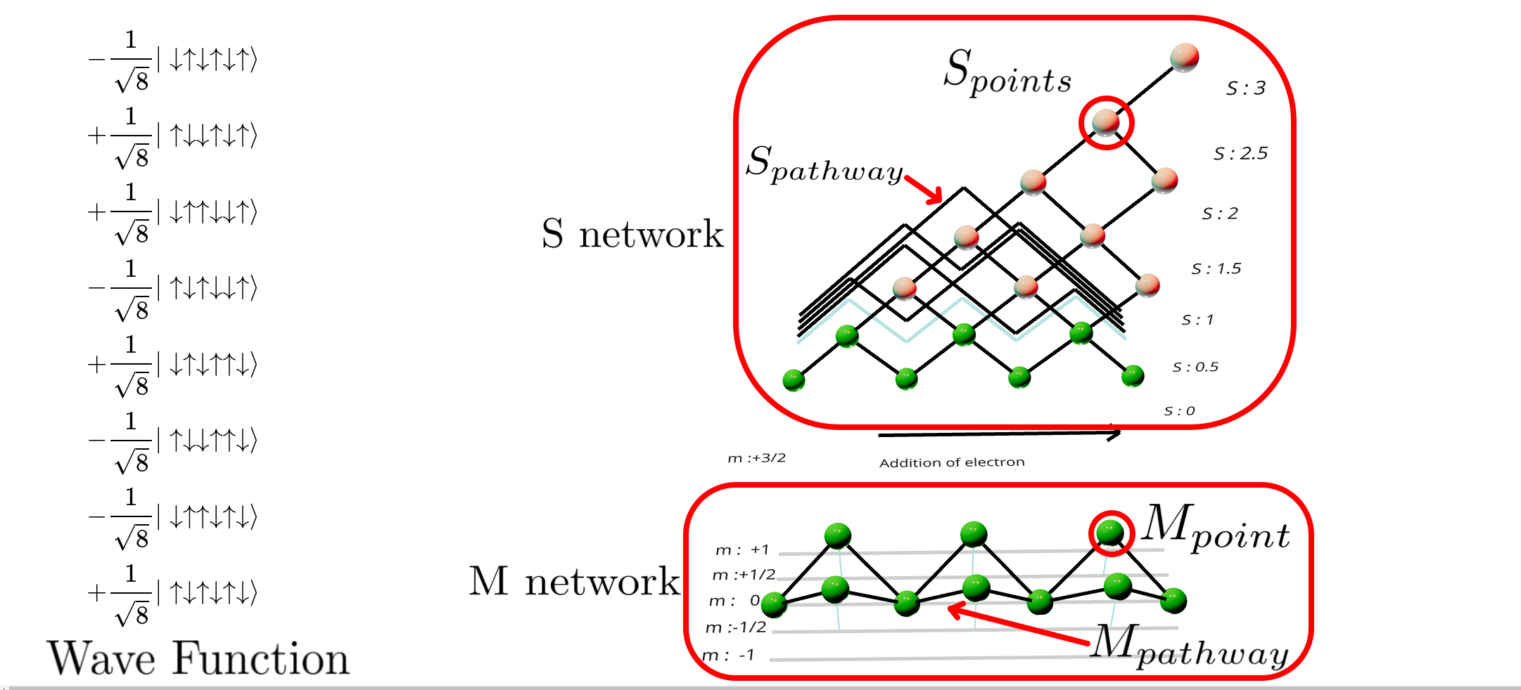
Wave Function Representation

The wave function with spin-only information is expressed as follows:

\( \vert \Psi^{S_{pathway}}_{(^{i}s)} \rangle = \sum^{M_{pathways}}_{k} CG_{k} \vert s_{1},m_{1} \rangle \otimes \dots \vert s_{n},m_{n} \rangle \)

Using creation operators, the wave function can be represented as:

\( \vert \Psi^{S_{pathway}}_{(^{i}s)} \rangle = \sum^{M_{pathways}}_{k} \sum_{k} CG_{k} C^{\dagger}_{\vert s,m\rangle_{j}} \dots \vert - \rangle \)

The Creation and annihilation operator is defined as: $$ a^{\dagger} = \begin{pmatrix} 0 & 0 \\ 1 & 0 \end{pmatrix} , a = \begin{pmatrix} 0 & 1 \\ 0 & 0 \end{pmatrix} $$

Creation operator for an electron in spatial orbtal \( \psi \)

\(\textbf{a}^{\dagger}_{\sigma \psi} = (\mathbf{s} \otimes ....\otimes \mathbf{s} \otimes a^{\dagger}_{\sigma } \otimes \unicode{x1D7D9}^{2} \otimes .... \otimes \unicode{x1D7D9}^{2})\psi. \)

\begin{equation} \begin{split} \left\langle\Psi_{m}\right|\hat{H}\left|\Psi_{n}\right\rangle = \sum_{i,j = 1}^{d}\sum_{s_{i},s_{j} = \uparrow,\downarrow}T_{ij}\left\langle\Psi_{m}\right|\textbf{a}_{i,s_{i}}^{\dagger}\textbf{a}_{j,s_{j}}\left|\Psi_{n}\right\rangle \\ + \frac{1}{2}\sum_{i,j,k,l = 1}^{d}\sum_{s_{i},s_{j},s_{k},s_{l} = \uparrow,\downarrow}V_{ijkl}\left\langle\Psi_{m}\right|\textbf{a}_{i,s_{i}}^{\dagger} \textbf{a}_{j,s_{j}}^{\dagger}\textbf{a}_{k,s_{k}} \textbf{a}_{l,s_{l}}\left|\Psi_{n}\right\rangle, \label{eq:coup} \end{split} \end{equation}

Singlet fission model for PDI trimer

A perylene diimide stack with three monomers (m, n, o) is considered.

HOMO and LUMO of each monomer are included.

Assuming singlet multiplicity, 19 diabatic states are constructed:

  • 1 ground state (GS)
  • 3 locally excited singlet states (LE)
  • 6 charge transfer states (CT)
  • 6 doubly excited mixed CT-triplet states
  • 3 correlated paired triplet states (1TT)

Example Wave Function

\begin{equation} | \text{S}_{1}\text{S}_{0}\text{S}_{0} \rangle = \substack{ \displaystyle{ - \frac { 1 }{ \sqrt { 8}}} \colorbox{yellow}{$ h_{m_{\uparrow} } l_{m_{\downarrow} } $ } \colorbox{green}{$ \color{white}{ h_{o_{\uparrow}} h_{o_{\downarrow}} h_{n_{\uparrow} } h_{n_{\downarrow}}} $} \displaystyle{ + \frac { 1 }{ \sqrt { 8}}} \colorbox{yellow}{$ h_{m_{\downarrow} } l_{m_{\uparrow} } $ } \colorbox{green}{$ \color{white}{ h_{o_{\uparrow}} h_{o_{\downarrow}} h_{n_{\uparrow} } h_{n_{\downarrow}}} $}\\ \displaystyle{ + \frac { 1 }{ \sqrt { 8}}} \colorbox{yellow}{$ h_{m_{\uparrow} } l_{m_{\downarrow} } $ } \colorbox{green}{$ \color{white}{ h_{o_{\downarrow}} h_{o_{\uparrow}} h_{n_{\uparrow} } h_{n_{\downarrow}}} $} \displaystyle{ - \frac { 1 }{ \sqrt { 8}}} \colorbox{yellow}{$ h_{m_{\downarrow} } l_{m_{\uparrow} } $ } \colorbox{green}{$ \color{white}{ h_{o_{\downarrow}} h_{o_{\uparrow}} h_{n_{\uparrow} } h_{n_{\downarrow}}} $}\\ \displaystyle{ + \frac { 1 }{ \sqrt { 8}}} \colorbox{yellow}{$ h_{m_{\uparrow} } l_{m_{\downarrow} } $ } \colorbox{green}{$ \color{white}{ h_{o_{\uparrow}} h_{o_{\downarrow}} h_{n_{\downarrow} } h_{n_{\uparrow}}} $} \displaystyle{ - \frac { 1 }{ \sqrt { 8}}} \colorbox{yellow}{$ h_{m_{\downarrow} } l_{m_{\uparrow} } $ } \colorbox{green}{$ \color{white}{ h_{o_{\uparrow}} h_{o_{\downarrow}} h_{n_{\downarrow} } h_{n_{\uparrow}}} $}\\ \displaystyle{ - \frac { 1 }{ \sqrt { 8}}} \colorbox{yellow}{$ h_{m_{\uparrow} } l_{m_{\downarrow} } $ } \colorbox{green}{$ \color{white}{ h_{o_{\downarrow}} h_{o_{\uparrow}} h_{n_{\downarrow} } h_{n_{\uparrow}}} $} \displaystyle{ + \frac { 1 }{ \sqrt { 8}}} \colorbox{yellow}{$ h_{m_{\downarrow} } l_{m_{\uparrow} } $ } \colorbox{green}{$ \color{white}{ h_{o_{\downarrow}} h_{o_{\uparrow}} h_{n_{\downarrow} } h_{n_{\uparrow}}} $} } \label{eq:LE} \end{equation}
\begin{equation} | \text{TS}_{0}\text{T} \rangle = \substack{ \displaystyle{ - \frac { 1 }{ \sqrt { 6}} } \colorbox{yellow}{ $ h_{m_{\uparrow}} l_{m_{\uparrow}} h_{o_{\downarrow}} l_{o_{\downarrow}} $ } \colorbox{green}{ $ \color{white}{ h_{n_{\uparrow}} h_{n_{\downarrow}}} $} \displaystyle{ - \frac { 1 }{ \sqrt { 6}} } \colorbox{yellow}{ $ h_{m_{\downarrow}} l_{m_{\downarrow}} h_{o_{\uparrow}} l_{o_{\uparrow}} $ } \colorbox{green}{ $ \color{white}{ h_{n_{\uparrow}} h_{n_{\downarrow}}} $}\\ \displaystyle{ + \frac { 1 }{ \sqrt { 6}} } \colorbox{yellow}{ $ h_{m_{\uparrow}} l_{m_{\uparrow}} h_{o_{\downarrow}} l_{o_{\downarrow}} $ } \colorbox{green}{ $ \color{white}{ h_{n_{\downarrow}} h_{n_{\uparrow}}} $} \displaystyle{ + \frac { 1 }{ \sqrt { 6}} } \colorbox{yellow}{ $ h_{m_{\downarrow}} l_{m_{\downarrow}} h_{o_{\uparrow}} l_{o_{\uparrow}} $ } \colorbox{green}{ $ \color{white}{ h_{n_{\downarrow}} h_{n_{\uparrow}}} $}\\ \displaystyle{ + \frac { 1 }{ \sqrt { 24}} } \colorbox{yellow}{ $ h_{m_{\uparrow}} l_{m_{\downarrow}} h_{o_{\uparrow}} l_{o_{\downarrow}} $ } \colorbox{green}{ $ \color{white}{ h_{n_{\uparrow}} h_{n_{\downarrow}}} $} \displaystyle{ + \frac { 1 }{ \sqrt { 24}} } \colorbox{yellow}{ $ h_{m_{\downarrow}} l_{m_{\uparrow}} h_{o_{\uparrow}} l_{o_{\downarrow}} $ } \colorbox{green}{ $ \color{white}{ h_{n_{\uparrow}} h_{n_{\downarrow}}} $}\\ \displaystyle{ + \frac { 1 }{ \sqrt { 24}} } \colorbox{yellow}{ $ h_{m_{\uparrow}} l_{m_{\downarrow}} h_{o_{\downarrow}} l_{o_{\uparrow}} $ } \colorbox{green}{ $ \color{white}{ h_{n_{\uparrow}} h_{n_{\downarrow}}} $} \displaystyle{ + \frac { 1 }{ \sqrt { 24}} } \colorbox{yellow}{ $ h_{m_{\downarrow}} l_{m_{\uparrow}} h_{o_{\downarrow}} l_{o_{\uparrow}} $ } \colorbox{green}{ $ \color{white}{ h_{n_{\uparrow}} h_{n_{\downarrow}}} $}\\ \displaystyle{ - \frac { 1 }{ \sqrt { 24}} } \colorbox{yellow}{ $ h_{m_{\uparrow}} l_{m_{\downarrow}} h_{o_{\uparrow}} l_{o_{\downarrow}} $ } \colorbox{green}{ $ \color{white}{ h_{n_{\downarrow}} h_{n_{\uparrow}}} $} \displaystyle{ - \frac { 1 }{ \sqrt { 24}} } \colorbox{yellow}{ $ h_{m_{\downarrow}} l_{m_{\uparrow}} h_{o_{\uparrow}} l_{o_{\downarrow}} $ } \colorbox{green}{ $ \color{white}{ h_{n_{\downarrow}} h_{n_{\uparrow}}} $}\\ \displaystyle{ - \frac { 1 }{ \sqrt { 24}} } \colorbox{yellow}{ $ h_{m_{\uparrow}} l_{m_{\downarrow}} h_{o_{\downarrow}} l_{o_{\uparrow}} $ } \colorbox{green}{ $ \color{white}{ h_{n_{\downarrow}} h_{n_{\uparrow}}} $} \displaystyle{ - \frac { 1 }{ \sqrt { 24}} } \colorbox{yellow}{ $ h_{m_{\downarrow}} l_{m_{\uparrow}} h_{o_{\downarrow}} l_{o_{\uparrow}} $ } \colorbox{green}{ $ \color{white}{ h_{n_{\downarrow}} h_{n_{\uparrow}}} $} } \label{eq:TST} \end{equation}

Couplings and Energies expressions

\begin{equation} \langle \text{TS}_{0}\text{T} \vert \hat{\text{T}} \vert \text{TS}_{0}\text{T} \rangle = 2\langle h_{n} | \hat{\text{h}} | h_{n} \rangle + \langle l_{m} | \hat{\text{h}} | l_{m} \rangle + \langle h_{m} | \hat{\text{h}} | h_{m} \rangle + \langle l_{o} | \hat{\text{h}} | l_{o} \rangle + \langle h_{o} | \hat{\text{h}} | h_{o} \rangle \label{eq:etst1} \end{equation} \begin{equation} \begin{split} \langle \text{TS}_{0}\text{T} \vert \hat{\text{G}} \vert \text{TS}_{0}\text{T} \rangle = & \colorbox{yellow}{$ + \frac{1}{2} (h_{m} h_{o} |h_{o} h_{m}) $ } \colorbox{yellow}{$ + \frac{1}{2} (h_{m} l_{o} |l_{o} h_{m}) $ }\\& \colorbox{yellow}{$ + \frac{1}{2} (h_{o} l_{m} |l_{m} h_{o}) $ } \colorbox{yellow}{$ + \frac{1}{2} (l_{m} l_{o} |l_{o} l_{m}) $ }\\& \colorbox{green}{$ \color{white}{+ (h_{m} h_{m} |h_{o} h_{o}) }$ } \colorbox{green}{$ \color{white}{+ (h_{m} h_{m} |l_{m} l_{m}) }$ }\\& \colorbox{green}{$ \color{white}{+ (h_{m} h_{m} |l_{o} l_{o}) }$ } \colorbox{green}{$ \color{white}{+ (h_{o} h_{o} |l_{m} l_{m}) }$ }\\& \colorbox{green}{$ \color{white}{+ (h_{o} h_{o} |l_{o} l_{o}) }$ } \colorbox{green}{$ \color{white}{+ (l_{m} l_{m} |l_{o} l_{o}) }$ }\\& \colorbox{orange}{$ + 2 (h_{n} h_{n} |h_{n} h_{n}) $ } \colorbox{orange}{$ + 2 (h_{m} h_{m} |h_{n} h_{n}) $ } \colorbox{orange}{$ + 2 (h_{o} h_{o} |h_{n} h_{n}) $ }\\& \colorbox{orange}{$ + 2 (h_{n} h_{n} |l_{m} l_{m}) $ } \colorbox{orange}{$ + 2 (h_{n} h_{n} |l_{o} l_{o}) $ }\\& \colorbox{pink}{$ - (h_{m} h_{n} |h_{n} h_{m}) $ } \colorbox{pink}{$ - (h_{m} l_{m} |l_{m} h_{m}) $ }\\& \colorbox{pink}{$ - (h_{o} h_{n} |h_{n} h_{o}) $ } \colorbox{pink}{$ - (h_{o} l_{o} |l_{o} h_{o}) $ }\\& \colorbox{pink}{$ - (h_{n} l_{m} |l_{m} h_{n}) $ } \colorbox{pink}{$ - (h_{n} l_{o} |l_{o} h_{n}) $ } \end{split} \label{eq:etst2} \end{equation}
\begin{equation} \langle \text{CAT} | \hat{\text{T}} | \text{S}_{0}\text{TT} \rangle = - \langle h_{m} | \hat{\text{h}} | h_{n} \rangle \label{eq:CAT_STT_1} \end{equation} \begin{equation} \begin{split} \langle \text{CAT} | \hat{\text{G}} | \text{S}_{0}\text{TT} \rangle = & \colorbox{yellow} { $ \frac{3}{2} (h_{m} h_{o} | h_{o} h_{n}) $} \colorbox{yellow} { $ +\frac{3}{2} (h_{m} l_{o} | l_{o} h_{n}) $}\\& \colorbox{green} {$ \color{white}{- (h_{m} h_{m} | h_{m} h_{n}) }$ } \colorbox{green} {$ \color{white}{- (h_{m} h_{n} | h_{n} h_{n}) }$ }\\& \colorbox{green} {$ \color{white}{- (h_{m} h_{n} | h_{o} h_{o}) }$ } \colorbox{green} {$ \color{white}{- (h_{m} h_{n} | l_{n} l_{n}) }$ } \colorbox{green} {$ \color{white}{- (h_{m} h_{n} | l_{o} l_{o}) }$ } \end{split} \label{eq:CAT_STT_2} \end{equation} \begin{equation} \langle \text{CAT} | \hat{\text{T}} | \text{TS}_{0}\text{T} \rangle = \langle l_{n} | \hat{\text{h}} | l_{m} \rangle \label{eq:CAT_TST_1} \end{equation} \begin{equation} \begin{split} \langle \text{CAT} | \hat{\text{G}} | \text{TS}_{0}\text{T} \rangle =& \colorbox{orange} { $ +2 (l_{m} l_{n} | h_{n} h_{n} ) $ }\\& \colorbox{yellow} { $ + \frac{1}{2} (l_{m} h_{o} | h_{o} l_{n} ) $ } \colorbox{yellow} { $ + \frac{1}{2} (l_{m} l_{o} | l_{o} l_{n} ) $ }\\& \colorbox{pink} { $ -(l_{m} h_{m} | h_{m} l_{n}) $ } \colorbox{pink} { $ -(l_{m} h_{n} | h_{n} l_{n}) $ }\\& \colorbox{green} { $ \color{white}{+ (l_{m} l_{n} | h_{m} h_{m} ) } $ } \colorbox{green} { $ \color{white}{+ (l_{m} l_{n} | h_{o} h_{o} ) } $ } \colorbox{green} { $ \color{white}{+ (l_{m} l_{n} | l_{o} l_{o} ) } $ } \end{split} \label{eq:CAT_TST_2} \end{equation}

incorporation of Core orbital Interaction

To incorporate the electron repulsion integrals (ERI) contribution of core electrons the electron repulsion interaction term (\(\text{G}_{core}\)) is determined by summing over specific core orbital indices in the expression involving the core density operator. The core density operator for the core orbitals is defined as: \begin{equation} \mathbf{\hat{D}}_{core} = 2 \mathbf{C}_{core} \mathbf{C}^{\dagger}_{core}, \label{eq:D_core} \end{equation} Thus, \begin{equation} \text{G}_{core} = \sum_{r,s } \mathbf{\hat{D}}_{core} [(pq|rs) - \frac{1}{2}(pr|sq)] \label{eq:V_core} \end{equation} The effective one-electron operator for active orbitals. \begin{equation} \hat{h}_{act} = \hat{h}^{AO} + \text{G}_{core}. \label{eq:h_act} \end{equation} \begin{equation} \langle \psi_{a} \vert \hat{h}^{MO} \vert \psi_{b} \rangle= \textbf{C}_{a}^{\dagger} \hat{h}_{\text{act}} \textbf{C}_{b} \label{eq:OneI} \end{equation} The ERI in the molecular orbital basis are calculated by transforming their counterparts in the atomic orbital (AO) basis: \begin{equation} ( \psi_{a} \psi_{b} \vert \psi_{c} \psi_{d} ) = \sum_{p}\sum_{q}\sum_{r}\sum_{s}C^{a}_{p}C^{b}_{q}C^{c}_{r}C^{d}_{s} (pq \vert rs) \label{eq:twoI} \end{equation}

Semi-Empirical AM1 Approximations

The implementation of \( T_{LE \rightarrow ^{1}TT} \) neglects additional two-electron contributions, and the following approximation was used:

\[ ^{Fock}T_{RP} = \sqrt{\frac{3}{2}}\left\vert \frac{( l_{A} | \mathbf{\hat{F}} | l_{B} ) ( l_{A} | \mathbf{\hat{F}} | h_{B} )}{\Delta E(\text{CA})} - \frac{( h_{A} | \mathbf{\hat{F}} | h_{B} ) ( h_{A} | \mathbf{\hat{F}} | l_{B} ) }{\Delta E(\text{AC})} \right\vert. \]

Then approximated by transitioning from Fock matrix elements to overlap matrix elements, represented as \(\langle \phi |\mathbf{\hat{F}}| \psi \rangle = \epsilon \langle \phi| \psi \rangle\), where \(\epsilon \) is constant. The obtained equation is: \begin{equation} ^{Overlap}T_{RP} = \sqrt{\frac{3}{2}}\left \vert\frac{\langle l_{A} | l_{B} \rangle \langle l_{A} | h_{B} \rangle}{\Delta E(\text{CA})} - \frac{\langle h_{A} | h_{B} \rangle \langle h_{A} | l_{B} \rangle }{\Delta E(\text{AC})}\right \vert. \end{equation}

Additionally, \(\Delta E(\text{CA})\) and \(\Delta E(\text{AC})\) are approximated as one for simplicity.

\begin{equation} T_{RP} = \left \vert \langle l_{A} | l_{B} \rangle \langle l_{A} | h_{B} \rangle - \langle h_{A} | h_{B} \rangle \langle h_{A} | l_{B} \rangle \right \vert. \end{equation}

Cofacially stacked perylene diimide (PDI) dimer molecules were analyzed.

The monomer geometry was optimized using the CAM-B3LYP functional, with an interplanar distance of \( \Delta Z = 3.41 \, \AA \).

The scan was conducted across spatial displacements \( \Delta X \): 0 to 4 \(\AA\), \( \Delta Y \): 0 to 4 \(\AA\), with a step size of 0.1 \(\AA\).

Semi-Empirical AM1 Approximations

PBI Diabatic Coupling

Benchmarking With Active Space Decomposition (ASD)

  • An ASD scan was performed using the RAS-CI/cc-pVDZ, employing a RAS(11,4,11)[1,1] configuration.
  • The ASD scan results are consistent with earlier studies by Mirjani et al. and Renaud et al.\(^{1,2}\)
  • Resemblance of Semi-Empirical scan to the ab-initio plot is excellent.
  • Non-Adiabatic Couplings

    By diagonalizing the diabatic Hamiltonian, the adiabatic states, denoted as \( |S^* \rangle \) and \( |TT^*\rangle \), are obtained.

    The singlet-fission rate is approximately proportional to the square of the first-order derivative coupling vector's magnitude.

    \[ \vec{\tau} = \langle S^* | \nabla | TT^*\rangle = \sum_{i=S_0S_1,S_1S_0,\ldots,TT} C^{\text{exciton}}_i \nabla C_i^{\text{triplet}} \] \[ \vert T_{RP} \vert^2_{\text{NAC}} = \frac{1}{2} \vert \langle {S^{\text{bright*}}} | \nabla | {TT^*} \rangle\vert^2 + \vert \langle {S^{\text{dark*}}} | \nabla | {TT^*} \rangle \vert^2 \]

    Shared features with scan of norm of non adiabatic coupling vector from Farag and Krylov

    • Used PySEQM for semi-empirical calculations.
    • PySEQM utilizes a PyTorch backend.
    • Automatic differentiation is employed for efficient gradient calculations.

    Autograd

    • Forward Mode:
      • Evaluates the computational graph during forward propagation.
      • Tracks operations and inputs for each variable.
    • Backward Mode:
      • Traverses the computational graph in reverse order during backpropagation.
      • Applies the chain rule to compute gradients efficiently.

    Functionality optimisation

    • The diabatic coupling \( T_{RP} \) is defined as: \( T_{RP} = \left \vert \langle l_{A} | l_{B} \rangle \langle l_{A} | h_{B} \rangle - \langle h_{A} | h_{B} \rangle \langle h_{A} | l_{B} \rangle \right \vert. \)

    • Functionality optimization using a custom objective function \( L(x) \).

    • The gradients for \( L(x) \) are computed automatically using an algorithmic differentiation framework, enabling efficient optimization.

    • The optimization minimizes the objective function \( L(x) \), which is expressed as: \( L(x) = E(x) - \omega \cdot \log(|T_{RP}|^2(x)). \)

    • The ground state energy component \( E(x) \) ensures that the molecular conformation is physically plausible

    Functionality optimisation

    By Johannes E Greiner and Anurag Singh

    • Searched for PBI dimer structures with high effective singlet fission coupling:
      • 500 optimizations conducted, followed by PCA to analyze resulting dimer structures.
      • Results grouped into 4 clusters based on structural characteristics:
        • Cluster 2:
          • Highest mean effective SF coupling.
          • Monomers have twist, stacking motif with translation in both the \( x \)- and \( y \)-directions, and rotation along the \( z \)-axis.
        • Cluster 3:
          • Exhibits curvature and strong translation along the \( x \)-axis.
        • Clusters 1 and 4:
          • Nearly planar structures.
          • Show rotation around the \( z \)-axis and relative translations of monomers in the \( x \)- and \( y \)-directions.
    Name \(2 E_{T_{1}} - E_{S_{1}}\) in eV
    PBI-C1\(_A\) -0.0682
    PBI-C1\(_B\) -0.0663
    PBI-C2\(_A\) -0.0795
    PBI-C2\(_B\) -0.0714
    Name \(2 E_{T_{1}} - E_{S_{1}}\) in eV
    PBI-C3\(_A\) 0.2993
    PBI-C3\(_B\) 0.3002
    PBI-C4\(_A\) -0.0676
    PBI-C4\(_B\) 0.2905
    PBI-Planar 0.3154

    Singlet Fission Study in B-N substituted perylene

    By Anurag Singh and Alexander Humeniuk

    The study aimed to increase the singlet fission rate through doping.

    1. Substitution Strategy:
      • All possible substitutions were enumerated where two adjacent carbon atoms were replaced by boron-nitrogen (B-N).
      • The resulting molecules were labeled as perylene-(BN)n-i, with:
        • \( n \): The number of B-N substitutions.
        • \( i = 0, 1, 2, \ldots \): Enumeration of structural isomers.
    2. Generated Molecules:
      • \((BN)_1\)-substitution resulted in 13 unique molecules.
      • \((BN)_2\)-substitution resulted in 256 unique molecules.
  • Property Calculations:
    • Vertical singlet and triplet excitation energies were computed at the CASPT2 and TD-DFT levels of theory.
  • Methodology:
    • Searched slipped stacking geometries of molecular dimers to achieve higher SF rates.
      • Diabatic method.
      • Non-Adiabatic Coupling (NAC) method.
  • Best Isomer

    • \(S_1\) excitation energy range: \( 1.8~\text{eV} \leq E(S_1, \text{CASPT2}) \leq 3.0~\text{eV} \).

      This ensures the molecule absorbs in then region where the solar spectrum has high intensity.

    • \(T_1\) state energy constraint:

      \( 0.8~\text{eV} < E(T_1, \text{TD-DFT}) \) To ensure solar cell operation with a singlet fission layer.

    • Condition for singlet fission energetics:

      Singlet fission must be exoergic or at most slightly endoergic. \( -0.3~\text{eV} < \Delta E_{ST}(\text{CASPT2}), \Delta E_{ST}(\text{TD-DFT}) < 0.2~\text{eV} \) pass this test.

    • \(T_2\) state constraint:

      The \(T_2 > S_1\) state to exclude intersystem crossing as a competing loss channel with singlet fission. The requirement is \( \Delta E_{TT}(\text{CASPT2}), \Delta E_{TT}(\text{TD-DFT}) < -0.2~\text{eV} \).

    • Only one candidate, BN2-112, remains.
    • BN2-112 has desirable properties, including:
      • A Lewis structure without formal charges.
      • Moderate biradical character of \( y_0 = 0.06 \), compared to a range of \( y_0 = 0.01 \) to \( 0.66 \) for the full set of isomers.
      • An oscillator strength \( f(S_0 \to S_1) = 0.27 \), which is close to undoped perylene (\( 0.30 \)).